Stochastic Computing#
The goal of this part of the workshop is to explore a simple example of stochastic computing with spiking neurons.
Step 0: Install Requirements#
First of all, we will need to install Norse. Please run the cell below. Read on while it’s running.
!pip install norse --quiet

import torch
import norse
Step 1: Neuron Model#
import numpy as np
import os


from norse.torch.module import LIFRefracRecurrentCell
from norse.torch.functional.threshold import superspike_fn
from norse.torch.functional.lif_refrac import (
    lif_refrac_feed_forward_step,
    lif_refrac_step,
)
from norse.torch.functional.lif_refrac import (
    LIFRefracFeedForwardState,
    LIFRefracState,
    LIFRefracParameters,
)
from norse.torch.functional.lif import LIFFeedForwardState, LIFState, LIFParameters
from norse.torch.functional.encode import poisson_encode


class LIFRefracNeurons(torch.nn.Module):
    def __init__(self, K, N):
        super(LIFRefracNeurons, self).__init__()

        self.K = K
        self.N = N

        self.v_leak = torch.nn.Parameter(
            1.0 * torch.ones(N, device=device), requires_grad=False
        )
        self.rho = torch.nn.Parameter(
            10.0 * torch.ones(N, device=device), requires_grad=False
        )
        lif_parameter = LIFParameters(
            v_leak=self.v_leak, method="super", alpha=torch.tensor(100)
        )
        lif_refrac = LIFRefracParameters(lif_parameter, self.rho)
        self.cell = LIFRefracRecurrentCell(K, N, p=lif_refrac)

    def forward(self, z):
        T, B, _ = z.shape
        s0 = LIFRefracState(
            LIFState(
                torch.zeros(B, self.N, device=z.device),
                0.9 * torch.ones(B, self.N, device=z.device),
                torch.zeros(B, N, device=z.device),
            ),
            torch.zeros(B, self.N, device=z.device),
        )
        refrac = []
        voltages = []

        for ts in range(T):
            output, s0 = self.cell(z[ts, :], s0)
            r = superspike_fn(s0.rho, torch.tensor(100.0, device=z.device))
            refrac.append(r)
            voltages.append(s0.lif.v)
        return torch.stack(refrac), torch.stack(voltages)
Step 2: Task#
The goal will be to approximate a binary probability distribution on three binary variables \(z_1, z_2, z_3\) represented by the refractory state \(\rho\) of three neurons. The correlation between the three refractory state variables can be computed in the following way
def three_point_correlations_func(rho):
    T, B, _ = rho.shape

    rb0 = torch.stack([1 - rho[:, :, 0], rho[:, :, 0]])
    rb1 = torch.stack([1 - rho[:, :, 1], rho[:, :, 1]])
    rb2 = torch.stack([1 - rho[:, :, 2], rho[:, :, 2]])
    return torch.einsum("atb,dtb,gtb -> badg", rb0, rb1, rb2) / T
Question (Optional): Can you think of a way how to implement this for an arbitrary number of neurons?
We will generate the target distribution by sampling from a population of refractory neurons, that way we can be reasonably sure that the model can be trained quickly to approximate the target distribution.
def generate_target_distribution(timesteps, batch_dimension, input_features):
    T, B, H = timesteps, batch_dimension, input_features
    z = poisson_encode(0.3 * torch.ones(B, H), T).detach().to(device)
    n_target = LIFRefracNeurons(H, N).to(device)
    refrac_t, voltages_t = n_target(z)
    readout_t = refrac_t[:, :, :5]
    p_target = three_point_correlations_func(readout_t).detach()
    p_target = p_target.flatten(start_dim=1)[0].unsqueeze(0).repeat(B, 1)
    return p_target
To plot the target we can use the following helper function
import matplotlib as mpl
import matplotlib.pyplot as plt


def target_plot(ax, p_target, width=0.35):
    ax.bar(np.arange(0, 8), p_target[0], width, label="$p_{t}$")
    ax.legend(loc="upper right")
    ax.set_xticks(np.arange(0, 8))
    ax.set_xticklabels(["{0:03b}".format(n) for n in np.arange(0, 8)], rotation=90)
    ax.set_ylabel("$p(z)$")
    ax.set_xlabel("$z$")
Now we generate a target distribution.
Once you’ve run the notebook to completion, you can consider doing one of the following Tasks:
Vary the number of timesteps, how to you expect fidelity of the approximation to behave?
Change the number of visible units (N) and number of poisson noise sources (H), what do you observe?
N = 32  # number of visible units
H = 256  # number of synapses connected to poisson noise sources
B = 32  # batch dimension
T = 1000  # number of timesteps to integrate (increase to get better sampling accuracy)
rho = 20  # refractory time in timesteps
device = "cpu"

p_target = generate_target_distribution(
    timesteps=T, batch_dimension=B, input_features=H
)
fig = plt.figure()
ax = fig.add_subplot()
target_plot(ax, p_target)
Step 3: Training#
The goal of the training procedure will be to minimize the Kullback-Leibler divergence between the target distribution \(p_t\) and the batch-averaged sampled distribution \(p_s\). In the machine-learning language the Kullback-Leibler divergence is one example of a loss-function and luckily PyTorch provides an implementation. This is another good example where relying on a widely used library saves us a lot of implementation time.
from tqdm.notebook import trange

neurons = LIFRefracNeurons(H, N).to(device)
optim = torch.optim.Adam(neurons.parameters())
losses = []

epochs = 40  # number of epochs to optimize
pbar = trange(epochs)

for i in pbar:
    optim.zero_grad()

    # sample new poisson noise for every iteration
    z = poisson_encode(0.3 * torch.ones(B, H), T).detach().to(device)

    # compute the refractory state and voltage traces
    refrac, voltages = neurons(z)

    # the first three neurons in each batch are our readout neurons
    readout = refrac[:, :, :3]

    # compute sampled probability distribution
    p_f = three_point_correlations_func(refrac).flatten(start_dim=1)

    # batch averaged Kullback-Leibler divergence
    loss = torch.nn.functional.kl_div(
        torch.log(p_f.clamp(min=1e-7)), p_target, reduction="batchmean"
    )

    # propagate gradient to parameters through time and take optimisation step
    loss.backward()
    optim.step()

    pbar.set_postfix({"loss": loss.detach().item()})
    losses.append(loss.detach().item())


# save all the training results
basepath = "results/stochastic"
os.makedirs(basepath, exist_ok=True)
np.save(os.path.join(basepath, "refrac.npy"), refrac.detach().numpy())
np.save(os.path.join(basepath, "p_target.npy"), p_target.detach().numpy())
np.save(os.path.join(basepath, "p_f.npy"), p_f.detach().numpy())
np.save(os.path.join(basepath, "losses.npy"), np.stack(losses))
np.save(os.path.join(basepath, "voltages.npy"), voltages.detach().numpy())
The model should converge to a loss of ~0.02-0.04.
Tasks / Questions:
What could be done to improve upon this result?
Change the input poisson noise, what happens?
Find out about different optimisers and try another one.
Step 4: Evaluating the Result#
Every scientist knows that a great plot is more than half of the reward.
basepath = "results/stochastic"

refrac = torch.tensor(np.load(os.path.join(basepath, "refrac.npy")))
p_target = torch.tensor(np.load(os.path.join(basepath, "p_target.npy")))
p_f = torch.tensor(np.load(os.path.join(basepath, "p_f.npy")))
losses = torch.tensor(np.load(os.path.join(basepath, "losses.npy")))
The following code is not really part of the workshop, but is necessary to create a decent (enough) looking figure of the results.
import matplotlib as mpl
import matplotlib.pyplot as plt
from matplotlib.collections import PatchCollection, LineCollection
from matplotlib.patches import Rectangle


def negedge(z, z_prev):
    return (1 - z) * z_prev


def posedge(z, z_prev):
    return z * (1 - z_prev)


mpl.rcParams["ytick.left"] = True
mpl.rcParams["ytick.labelleft"] = True
mpl.rcParams["axes.spines.left"] = True
mpl.rcParams["axes.spines.right"] = False
mpl.rcParams["axes.spines.top"] = False
mpl.rcParams["axes.spines.bottom"] = True
mpl.rcParams["legend.frameon"] = False


def sampling_figure(ax, refrac):
    T, _, _ = refrac.shape
    N = 3

    posedges = []
    negedges = []

    z_prev = torch.zeros_like(refrac[0])
    z = refrac[0, :]

    ax.set_yticks(1.2 * np.arange(0, 5) + 0.6)
    ax.set_yticklabels(["$z_1$", "$z_2$", "$z_3$", "$z_4$", "$z_5$"])
    ax.spines["left"].set_visible(False)

    for ts in range(T):
        z = refrac[ts]
        posedges.append(posedge(z, z_prev))
        negedges.append(negedge(z, z_prev))
        z_prev = z

    posedges = torch.stack(posedges)
    negedges = torch.stack(negedges)

    lines = []
    rects = []

    facecolor = "black"

    for k in range(N):
        t = posedges[200:400, 0, k].to_sparse().coalesce().indices()[0]
        t_r = negedges[200:400, 0, k].to_sparse().coalesce().indices()[0]

        for ts, tf in zip(t, t_r):
            rect = Rectangle((ts, k * 1.2), tf - ts, 1.0)
            line = [(ts, k * 1.2), (ts, k * 1.2 + 1.0)]
            rects.append(rect)
            lines.append(line)

    pc = PatchCollection(rects, facecolor=facecolor, alpha=0.2, edgecolor=None)
    lc = LineCollection(lines, color="black")

    for k in range(N):
        ax.plot(voltages[200:400, 0, k].detach() + k * 1.2, label=f"$v_{k}$")

    ax.add_collection(pc)
    ax.set_ylabel("Neuron")
    ax.set_xlabel("T [ms]")
    # ax.add_collection(lc)
    ax.legend(loc="upper right", bbox_to_anchor=(1.15, 1))


def figure_stochastic_computing(p_f, p_target, losses, refrac):
    width = 0.35

    fig = plt.figure(constrained_layout=True, figsize=(7, 9))
    gs = fig.add_gridspec(nrows=3, ncols=1)

    ax_sampling = fig.add_subplot(gs[0, 0])
    ax_prob = fig.add_subplot(gs[1, 0])
    ax_loss = fig.add_subplot(gs[2, 0])

    p_f_mean = np.mean(p_f.detach().numpy(), axis=0)
    p_f_min = np.min(p_f.detach().numpy(), axis=0)
    p_f_max = np.max(p_f.detach().numpy(), axis=0)

    ax_sampling.text(
        -0.1, 1.1, "A", transform=ax_sampling.transAxes, size="medium", weight="normal"
    )
    sampling_figure(ax_sampling, refrac)

    # plot the probabilities

    ax_prob.text(
        -0.1, 1.1, "B", transform=ax_prob.transAxes, size="medium", weight="normal"
    )
    ax_prob.bar(
        np.arange(0, 8) - width / 2, p_f[0].detach().numpy(), width, label="$p_s$"
    )
    ax_prob.bar(np.arange(0, 8) + width / 2, p_target[0], width, label="$p_{t}$")
    ax_prob.legend(loc="upper right")
    ax_prob.set_xticks(np.arange(0, 8))
    ax_prob.set_xticklabels(["{0:03b}".format(n) for n in np.arange(0, 8)], rotation=90)
    ax_prob.set_ylabel("$p(z)$")
    ax_prob.set_xlabel("$z$")
    ax_prob.errorbar(
        np.arange(0, 8) - width / 2,
        p_f_mean,
        yerr=[p_f_mean - p_f_min, p_f_max - p_f_mean],
        color="r",
        fmt=".k",
    )

    ax_loss.text(
        -0.1, 1.1, "C", transform=ax_loss.transAxes, size="medium", weight="normal"
    )
    ax_loss.semilogy(losses)
    ax_loss.set_ylabel("$KL(p_s | p_t)$")
    ax_loss.set_xlabel("Epoch")
    return fig
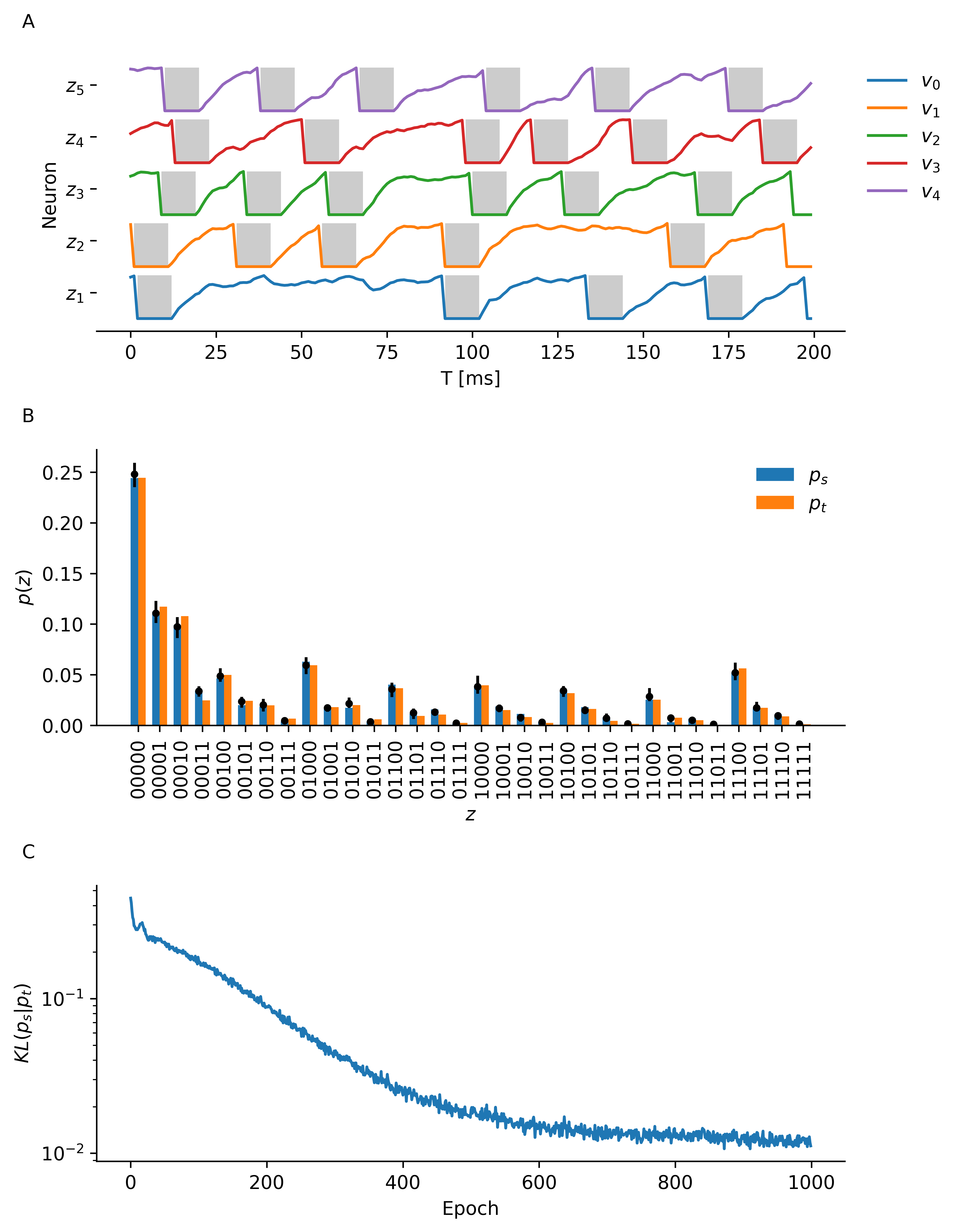
The resulting plot shows part of the neuron membrane traces of the three readout neurons, the value of the binary refractory state variables is indicated by gray shading (A). We also see how well the sampled distribution approximates the target distribution (B). Finally we plot the Kulback-Leibler divergence (C).
fig = figure_stochastic_computing(p_f, p_target, losses, refrac)
fig.savefig("stochastic_computing.png", dpi=600, bbox_inches="tight")
The same kind of experiment can be repeated for 5 variables. Below is an example of one such run.