Training an MNIST classifier

Norse is a library where you can simulate neural networks that are driven by atomic and sparse events over time, rather than large and dense tensors without time.

Outcomes: This tutorial introduces the “Hello World” task of deep-learning: How to classify hand-written digits using norse

1. Installation

import torch
import numpy as np
import matplotlib.pyplot as plt

We can simply install Norse through pip:

!pip install --quiet norse

2. Spiking neurons

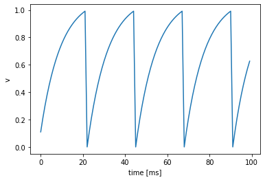
Spiking neuron models are given as (typically very simple) systems of ordinary differential equations. A common example used is the so called current based leaky integrate and fire neuron model (LIF). Its differential equation is given by \begin{align*} \dot{v} &= -(v - v_\text{reset}) + I \ \dot{I} &= -I + I_\text{in} \end{align*} together with jump and transition equations, that specify when a jump occurs and how the state variables change. A prototypical equation is a leaky integrator with constant current input \(I_\text{in}\), with jump condition \(v - 1 = 0\) and transition equation \(v^+ - v^- = -1\).

from norse.torch.functional import (
    lif_step,
    lift,
    lif_feed_forward_step,
    lif_current_encoder,
    LIFParameters,
)

N = 1  # number of neurons to consider
T = 100  # number of timesteps to integrate

p = LIFParameters()
v = torch.zeros(N)  # initial membrane voltage
input_current = 1.1 * torch.ones(N)

voltages = []

for ts in range(T):
    z, v = lif_current_encoder(input_current, v, p)
    voltages.append(v)

voltages = torch.stack(voltages)

We can now plot the voltages over time:

plt.ylabel("v")
plt.xlabel("time [ms]")
plt.plot(voltages)

[<matplotlib.lines.Line2D at 0x7f995f3a6310>]

3. MNIST Task

A common toy dataset to test machine learning approaches on is the MNIST handwritten digit recognition dataset. The goal is to distinguish handwritten digits 0..9 based on a 28x28 grayscale picture. Run the cell below to download the training and test data for MNIST.

import torchvision

BATCH_SIZE = 256

transform = torchvision.transforms.Compose(
    [
        torchvision.transforms.ToTensor(),
        torchvision.transforms.Normalize((0.1307,), (0.3081,)),
    ]
)

train_data = torchvision.datasets.MNIST(
    root=".",
    train=True,
    download=True,
    transform=transform,
)

train_loader = torch.utils.data.DataLoader(
    train_data, batch_size=BATCH_SIZE, shuffle=True
)

test_loader = torch.utils.data.DataLoader(
    torchvision.datasets.MNIST(
        root=".",
        train=False,
        transform=transform,
    ),
    batch_size=BATCH_SIZE,
)

Downloading http://yann.lecun.com/exdb/mnist/train-images-idx3-ubyte.gz
Downloading http://yann.lecun.com/exdb/mnist/train-images-idx3-ubyte.gz to ./MNIST/raw/train-images-idx3-ubyte.gz

Extracting ./MNIST/raw/train-images-idx3-ubyte.gz to ./MNIST/raw

Downloading http://yann.lecun.com/exdb/mnist/train-labels-idx1-ubyte.gz
Downloading http://yann.lecun.com/exdb/mnist/train-labels-idx1-ubyte.gz to ./MNIST/raw/train-labels-idx1-ubyte.gz

Extracting ./MNIST/raw/train-labels-idx1-ubyte.gz to ./MNIST/raw

Downloading http://yann.lecun.com/exdb/mnist/t10k-images-idx3-ubyte.gz
Downloading http://yann.lecun.com/exdb/mnist/t10k-images-idx3-ubyte.gz to ./MNIST/raw/t10k-images-idx3-ubyte.gz

Extracting ./MNIST/raw/t10k-images-idx3-ubyte.gz to ./MNIST/raw

Downloading http://yann.lecun.com/exdb/mnist/t10k-labels-idx1-ubyte.gz
Downloading http://yann.lecun.com/exdb/mnist/t10k-labels-idx1-ubyte.gz to ./MNIST/raw/t10k-labels-idx1-ubyte.gz

Extracting ./MNIST/raw/t10k-labels-idx1-ubyte.gz to ./MNIST/raw

3.1 Encoding Input Data

One of the distinguishing features of spiking neural networks is that they operate on temporal data encoded as spikes. Common datasets in machine learning of course don’t use such an encoding and therefore make a encoding step necessary. Here we choose to treat the grayscale value of an MNIST image as a constant current to produce input spikes to the rest of the network. Another option would be to interpret the grayscale value as a spike probabilty at each timestep.

Constant Current Encoder

from norse.torch import ConstantCurrentLIFEncoder

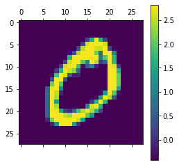
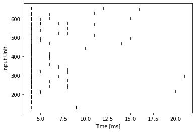
We can easily visualise the effect of this choice of encoding on a sample image in the training data set

img, label = train_data[1]

plt.matshow(img[0])
plt.colorbar()
print(label)

0

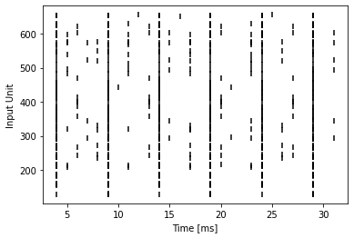
T = 32
example_encoder = ConstantCurrentLIFEncoder(T)


example_input = example_encoder(img)
example_spikes = example_input.reshape(T, 28 * 28).to_sparse().coalesce()
t = example_spikes.indices()[0]
n = example_spikes.indices()[1]

plt.scatter(t, n, marker="|", color="black")
plt.ylabel("Input Unit")
plt.xlabel("Time [ms]")
plt.show()

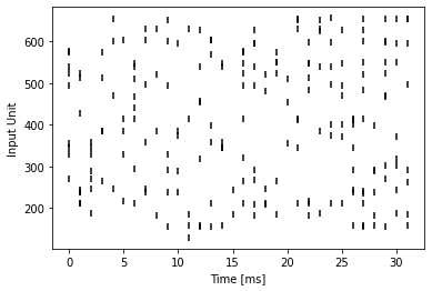
Poisson Encoding

As can be seen from the spike raster plot, this kind of encoding does not produce spike patterns which are necessarily biologically realistic. We could rectify this situation by employing cells with varying threshholds and a finer integration time step. Alternatively we can encode the grayscale input images into poisson spike trains

from norse.torch import PoissonEncoder

This produces a more biological plausible input pattern, as can be seen below:

T = 32
example_encoder = PoissonEncoder(T, f_max=20)

example_input = example_encoder(img)
example_spikes = example_input.reshape(T, 28 * 28).to_sparse().coalesce()
t = example_spikes.indices()[0]
n = example_spikes.indices()[1]

plt.scatter(t, n, marker="|", color="black")
plt.ylabel("Input Unit")
plt.xlabel("Time [ms]")
plt.show()

Spike Latency Encoding

Yet another example is a spike latency encoder. In this case each input neuron spikes only once, the first time the input crosses the threshhold.

from norse.torch import SpikeLatencyLIFEncoder

T = 32
example_encoder = SpikeLatencyLIFEncoder(T)


example_input = example_encoder(img)
example_spikes = example_input.reshape(T, 28 * 28).to_sparse().coalesce()
t = example_spikes.indices()[0]
n = example_spikes.indices()[1]

plt.scatter(t, n, marker="|", color="black")
plt.ylabel("Input Unit")
plt.xlabel("Time [ms]")
plt.show()

3.2 Defining a Network

Once the data is encoded into spikes, a spiking neural network can be constructed in the same way as a one would construct a recurrent neural network. Here we define a spiking neural network with one recurrently connected layer with hidden_features LIF neurons and a readout layer with output_features and leaky-integrators. As you can see, we can freely combine spiking neural network primitives with ordinary torch.nn.Module layers.

from norse.torch import LIFParameters, LIFState
from norse.torch.module.lif import LIFCell, LIFRecurrentCell

# Notice the difference between "LIF" (leaky integrate-and-fire) and "LI" (leaky integrator)
from norse.torch import LICell, LIState

from typing import NamedTuple


class SNNState(NamedTuple):
    lif0: LIFState
    readout: LIState


class SNN(torch.nn.Module):
    def __init__(
        self, input_features, hidden_features, output_features, record=False, dt=0.001
    ):
        super(SNN, self).__init__()
        self.l1 = LIFRecurrentCell(
            input_features,
            hidden_features,
            p=LIFParameters(alpha=100, v_th=torch.tensor(0.5)),
            dt=dt,
        )
        self.input_features = input_features
        self.fc_out = torch.nn.Linear(hidden_features, output_features, bias=False)
        self.out = LICell(dt=dt)

        self.hidden_features = hidden_features
        self.output_features = output_features
        self.record = record

    def forward(self, x):
        seq_length, batch_size, _, _, _ = x.shape
        s1 = so = None
        voltages = []

        if self.record:
            self.recording = SNNState(
                LIFState(
                    z=torch.zeros(seq_length, batch_size, self.hidden_features),
                    v=torch.zeros(seq_length, batch_size, self.hidden_features),
                    i=torch.zeros(seq_length, batch_size, self.hidden_features),
                ),
                LIState(
                    v=torch.zeros(seq_length, batch_size, self.output_features),
                    i=torch.zeros(seq_length, batch_size, self.output_features),
                ),
            )

        for ts in range(seq_length):
            z = x[ts, :, :, :].view(-1, self.input_features)
            z, s1 = self.l1(z, s1)
            z = self.fc_out(z)
            vo, so = self.out(z, so)
            if self.record:
                self.recording.lif0.z[ts, :] = s1.z
                self.recording.lif0.v[ts, :] = s1.v
                self.recording.lif0.i[ts, :] = s1.i
                self.recording.readout.v[ts, :] = so.v
                self.recording.readout.i[ts, :] = so.i
            voltages += [vo]

        return torch.stack(voltages)

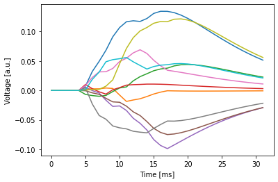
We can visualize the output produced by the recurrent spiking neural network on the example input.

example_snn = SNN(28 * 28, 100, 10, record=True, dt=0.001)

example_readout_voltages = example_snn(example_input.unsqueeze(1))
voltages = example_readout_voltages.squeeze(1).detach().numpy()

plt.plot(voltages)
plt.ylabel("Voltage [a.u.]")
plt.xlabel("Time [ms]")
plt.show()

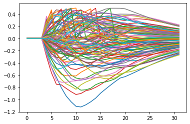
plt.plot(example_snn.recording.lif0.v.squeeze(1).detach().numpy())
plt.show()

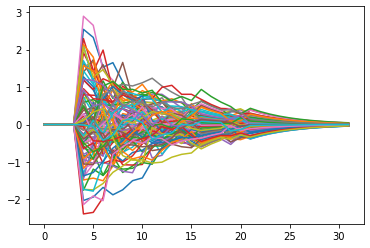
plt.plot(example_snn.recording.lif0.i.squeeze(1).detach().numpy())
plt.show()

3.3 Decoding the Output

The output of the network we have defined are \(10\) membrane voltage traces. What remains to do is to interpret those as a probabilty distribution. One way of doing so is to determine the maximum along the time dimension and to then compute the softmax of these values. There are other options of course, for example to consider the average membrane voltage in a given time window or use a LIF neuron output layer and consider the time to first spike.

def decode(x):
    x, _ = torch.max(x, 0)
    log_p_y = torch.nn.functional.log_softmax(x, dim=1)
    return log_p_y

An alternative way of decoding would be to consider only the membrane trace at the last measured time step.

def decode_last(x):
    x = x[-1]
    log_p_y = torch.nn.functional.log_softmax(x, dim=1)
    return log_p_y

3.4 Training the Network

The final model is then simply the sequential composition of these three steps: Encoding, a spiking neural network and decoding.

class Model(torch.nn.Module):
    def __init__(self, encoder, snn, decoder):
        super(Model, self).__init__()
        self.encoder = encoder
        self.snn = snn
        self.decoder = decoder

    def forward(self, x):
        x = self.encoder(x)
        x = self.snn(x)
        log_p_y = self.decoder(x)
        return log_p_y

We can then instantiate the model with the recurrent SNN network defined above.

T = 32
LR = 0.002
INPUT_FEATURES = 28 * 28
HIDDEN_FEATURES = 100
OUTPUT_FEATURES = 10

if torch.cuda.is_available():
    DEVICE = torch.device("cuda")
else:
    DEVICE = torch.device("cpu")

model = Model(
    encoder=ConstantCurrentLIFEncoder(
        seq_length=T,
    ),
    snn=SNN(
        input_features=INPUT_FEATURES,
        hidden_features=HIDDEN_FEATURES,
        output_features=OUTPUT_FEATURES,
    ),
    decoder=decode,
).to(DEVICE)

optimizer = torch.optim.Adam(model.parameters(), lr=LR)
model

Model(
  (encoder): ConstantCurrentLIFEncoder()
  (snn): SNN(
    (l1): LIFRecurrentCell(input_size=784, hidden_size=100, p=LIFParameters(tau_syn_inv=tensor(200.), tau_mem_inv=tensor(100.), v_leak=tensor(0.), v_th=tensor(0.5000), v_reset=tensor(0.), method='super', alpha=tensor(100)), autapses=False, dt=0.001)
    (fc_out): Linear(in_features=100, out_features=10, bias=False)
    (out): LICell(p=LIParameters(tau_syn_inv=tensor(200.), tau_mem_inv=tensor(100.), v_leak=tensor(0.)), dt=0.001)
  )
)

What remains to do is to setup training and test code. This code is completely independent of the fact that we are training a spiking neural network and in fact has been largely copied from the pytorch tutorials.

from tqdm.notebook import tqdm, trange

EPOCHS = 5  # Increase this number for better performance


def train(model, device, train_loader, optimizer, epoch, max_epochs):
    model.train()
    losses = []

    for (data, target) in tqdm(train_loader, leave=False):
        data, target = data.to(device), target.to(device)
        optimizer.zero_grad()
        output = model(data)
        loss = torch.nn.functional.nll_loss(output, target)
        loss.backward()
        optimizer.step()
        losses.append(loss.item())

    mean_loss = np.mean(losses)
    return losses, mean_loss

Just like the training function, the test function is standard boilerplate, common with any other supervised learning task.

def test(model, device, test_loader, epoch):
    model.eval()
    test_loss = 0
    correct = 0
    with torch.no_grad():
        for data, target in test_loader:
            data, target = data.to(device), target.to(device)
            output = model(data)
            test_loss += torch.nn.functional.nll_loss(
                output, target, reduction="sum"
            ).item()  # sum up batch loss
            pred = output.argmax(
                dim=1, keepdim=True
            )  # get the index of the max log-probability
            correct += pred.eq(target.view_as(pred)).sum().item()

    test_loss /= len(test_loader.dataset)

    accuracy = 100.0 * correct / len(test_loader.dataset)

    return test_loss, accuracy

training_losses = []
mean_losses = []
test_losses = []
accuracies = []

torch.autograd.set_detect_anomaly(True)

for epoch in trange(EPOCHS):
    training_loss, mean_loss = train(
        model, DEVICE, train_loader, optimizer, epoch, max_epochs=EPOCHS
    )
    test_loss, accuracy = test(model, DEVICE, test_loader, epoch)
    training_losses += training_loss
    mean_losses.append(mean_loss)
    test_losses.append(test_loss)
    accuracies.append(accuracy)

print(f"final accuracy: {accuracies[-1]}")

final accuracy: 94.5

We can visualize the output of the trained network on an example input

trained_snn = model.snn.cpu()
trained_readout_voltages = trained_snn(example_input.unsqueeze(1))
plt.plot(trained_readout_voltages.squeeze(1).detach().numpy())

plt.ylabel("Voltage [a.u.]")
plt.xlabel("Time [ms]")
plt.show()

That’s your first MNIST classification task done using a trained Spiking Neural Network! As you must have seen the only difference was to change the data into a format compatible for SNNs, i.e. ‘spikes’ and adding LIF neuron layers in a regular PyTorch framework of building a Neural Network.

4. Modifying the Network

We can change how the SNN behaves by modifying different aspects of the Network, the crucial ones are discussed below

4.1 Encoding and Decoding Scheme

There are alternative ways of encoding and decoding the data to and from spikes as discussed previously. Here we go through two such alternative with the same network we’ve used before.

As is the the outer training loop.

import importlib
from norse.torch.module import encode

encode = importlib.reload(encode)

# from norse.torch.module import encode

T = 32
LR = 0.002
INPUT_FEATURES = 28 * 28
HIDDEN_FEATURES = 100
OUTPUT_FEATURES = 10

if torch.cuda.is_available():
    DEVICE = torch.device("cuda")
else:
    DEVICE = torch.device("cpu")

model = Model(
    encoder=encode.SpikeLatencyLIFEncoder(T),
    snn=SNN(
        input_features=INPUT_FEATURES,
        hidden_features=HIDDEN_FEATURES,
        output_features=OUTPUT_FEATURES,
    ),
    decoder=decode,
).to(DEVICE)

optimizer = torch.optim.Adam(model.parameters(), lr=LR)
model

training_losses = []
mean_losses = []
test_losses = []
accuracies = []

for epoch in trange(EPOCHS):
    training_loss, mean_loss = train(
        model, DEVICE, train_loader, optimizer, epoch, max_epochs=EPOCHS
    )
    test_loss, accuracy = test(model, DEVICE, test_loader, epoch)
    training_losses += training_loss
    mean_losses.append(mean_loss)
    test_losses.append(test_loss)
    accuracies.append(accuracy)

print(f"final accuracy: {accuracies[-1]}")

Network with Poisson Encoded Input

T = 32
LR = 0.002
INPUT_FEATURES = 28 * 28
HIDDEN_FEATURES = 100
OUTPUT_FEATURES = 10

if torch.cuda.is_available():
    DEVICE = torch.device("cuda")
else:
    DEVICE = torch.device("cpu")

model = Model(
    encoder=encode.PoissonEncoder(T, f_max=20),
    snn=SNN(
        input_features=INPUT_FEATURES,
        hidden_features=HIDDEN_FEATURES,
        output_features=OUTPUT_FEATURES,
    ),
    decoder=decode,
).to(DEVICE)

optimizer = torch.optim.Adam(model.parameters(), lr=LR)
model

training_losses = []
mean_losses = []
test_losses = []
accuracies = []

for epoch in trange(EPOCHS):
    training_loss, mean_loss = train(
        model, DEVICE, train_loader, optimizer, epoch, max_epochs=EPOCHS
    )
    test_loss, accuracy = test(model, DEVICE, test_loader, epoch)
    training_losses += training_loss
    mean_losses.append(mean_loss)
    test_losses.append(test_loss)
    accuracies.append(accuracy)
    # print(f"epoch: {epoch}, mean_loss: {mean_loss}, test_loss: {test_loss}, accuracy: {accuracy}", flush=True)

print(f"final accuracy: {accuracies[-1]}")

As can be seen from the training result, this combination of hyperparameters, decoding and encoding scheme performs worse than the alternative we’ve presented before. As with any machine learning approach one of the biggest challenges is to find a combination of these choices that works well. Sometimes theoretical knowledge helps in making these choices. For example it is well known that poisson encoded input will converge with \(1/\sqrt{T}\), where \(T\) is the number of timesteps. So most likely the low number of timesteps (\(T = 32\)) contributes to the poor performance.

In the next section we will see that choice of network architecture is also key in training performant spiking neural networks, just as it is for artifiicial neural networks.

4.2 Convolutional Networks

The simple two layer recurrent spiking neural network we’ve defined above achieves a respectable ~96.5% accuracy after 10 training epochs. One common way to improve on this performance is to use convolutional neural networks. We define here two convolutional layers and one spiking classification layer. Just as in the recurrent spiking neural network before, we use a non-spiking leaky integrator for readout.

The torch.nn.functional.max_pool2d on binary values is a logical or operation on its inputs.

from norse.torch.module.leaky_integrator import LILinearCell
from norse.torch.functional.lif import LIFFeedForwardState
from norse.torch.functional.leaky_integrator import LIState

from typing import NamedTuple


class ConvNet(torch.nn.Module):
    def __init__(self, num_channels=1, feature_size=28, method="super", alpha=100):
        super(ConvNet, self).__init__()

        self.features = int(((feature_size - 4) / 2 - 4) / 2)

        self.conv1 = torch.nn.Conv2d(num_channels, 20, 5, 1)
        self.conv2 = torch.nn.Conv2d(20, 50, 5, 1)
        self.fc1 = torch.nn.Linear(self.features * self.features * 50, 500)
        self.lif0 = LIFCell(p=LIFParameters(method=method, alpha=alpha))
        self.lif1 = LIFCell(p=LIFParameters(method=method, alpha=alpha))
        self.lif2 = LIFCell(p=LIFParameters(method=method, alpha=alpha))
        self.out = LILinearCell(500, 10)

    def forward(self, x):
        seq_length = x.shape[0]
        batch_size = x.shape[1]

        # specify the initial states
        s0 = s1 = s2 = so = None

        voltages = torch.zeros(
            seq_length, batch_size, 10, device=x.device, dtype=x.dtype
        )

        for ts in range(seq_length):
            z = self.conv1(x[ts, :])
            z, s0 = self.lif0(z, s0)
            z = torch.nn.functional.max_pool2d(z, 2, 2)
            z = 10 * self.conv2(z)
            z, s1 = self.lif1(z, s1)
            z = torch.nn.functional.max_pool2d(z, 2, 2)
            z = z.view(-1, 4**2 * 50)
            z = self.fc1(z)
            z, s2 = self.lif2(z, s2)
            v, so = self.out(torch.nn.functional.relu(z), so)
            voltages[ts, :, :] = v
        return voltages

img, label = train_data[2]

plt.matshow(img[0])
plt.show()
print(label)

Just as we did we can visualise the output of the untrained convolutional network on a sample input. Notice that compared to the previous untrained output the first non-zero membrane trace values appear later. This is due to the fact that there is a finite delay for each added layer in the network.

T = 48
example_encoder = encode.ConstantCurrentLIFEncoder(T)
example_input = example_encoder(img)
example_snn = ConvNet()
example_readout_voltages = example_snn(example_input.unsqueeze(1))

plt.plot(example_readout_voltages.squeeze(1).detach().numpy())
plt.ylabel("Voltage [a.u.]")
plt.xlabel("Time [ms]")
plt.show()

T = 48
LR = 0.001
EPOCHS = 5  # Increase this for improved accuracy

if torch.cuda.is_available():
    DEVICE = torch.device("cuda")
else:
    DEVICE = torch.device("cpu")

model = Model(
    encoder=encode.ConstantCurrentLIFEncoder(T), snn=ConvNet(alpha=80), decoder=decode
).to(DEVICE)

optimizer = torch.optim.Adam(model.parameters(), lr=LR)
model

training_losses = []
mean_losses = []
test_losses = []
accuracies = []

for epoch in trange(EPOCHS):
    training_loss, mean_loss = train(
        model, DEVICE, train_loader, optimizer, epoch, max_epochs=EPOCHS
    )
    test_loss, accuracy = test(model, DEVICE, test_loader, epoch)
    training_losses += training_loss
    mean_losses.append(mean_loss)
    test_losses.append(test_loss)
    accuracies.append(accuracy)

print(f"final accuracy: {accuracies[-1]}")

trained_snn = model.snn.cpu()

trained_readout_voltages = trained_snn(example_input.unsqueeze(1))

print(trained_readout_voltages.shape)

for i in range(10):
    plt.plot(
        trained_readout_voltages[:, :, i].squeeze(1).detach().numpy(), label=f"{i}"
    )

plt.ylabel("Voltage [a.u.]")
plt.xlabel("Time [ms]")
plt.legend()
plt.show()

As we can see the output neuron for the label ‘4’ indeed integrates the largest number of spikes.

plt.matshow(np.squeeze(img, 0))

5. Conclusions

We’ve seen that on a small supervised learning task it is relatively easy to define spiking neural networks that perform about as well as non-spiking artificial networks. The network architecture used is in direct correspondence to one that would be used to solve such a task with an artificial neural network, with the non-linearities replaced by spiking units.

The remaining difference in performance might be related to a number of choices:

• hyperparameters of the optimizer

• precise architecture (e.g. dimensionality of the classification layer)

• weight initialisation

• decoding scheme

• encoding scheme

• number of integration timesteps

The first three points are in common with the problems encountered in the design and training of artificial neural network classifiers. Comparatively little is known though about their interplay for spiking neural network architectures.

The last three points are special to spiking neural network problems simply because of their constraints on what kind of data they can process naturally. While their interplay has certainly been investigated in the literature, it is unclear if there is a good answer what encoding and decoding should be chosen in general.

Finally we’ve also omitted any regularisation or data-augementation, which could further improve performance. Common techniques would be to introduce weight decay or penalise unbiologically high firing rates. In the simplest case those can enter as addtional terms in the loss function we’ve defined above.

---

We have plenty more resources in our notebook repository if you’re feeling adventurous. Also, our documentation tells you much more about what Norse is and why we built it at: https://norse.github.io/norse/

Don’t forget to join our Discord server and to support us by either donating or contributing your work upstream. Norse is open-source and built with love for the community. We couldn’t do it without your help!