Spiking neural networks with Norse#
Norse is a library where you can simulate neural networks that are driven by atomic and sparse events over time, rather than large and dense tensors without time.
These event-driven (or spike-driven) neural networks are interesting for two reasons: 1) they are extremely energy- and compute efficient when run on the correct hardware and 2) they work in the same way that the human brain operates.
Note
You can execute the notebooks on this website by hitting above and pressing Live Code.
Outcomes: In this notebook, you will learn to setup spiking neuron layers and train the network using Norse and PyTorch.
Before you continue with this notebook, we strongly recommend you familiarize yourself with PyTorch (at least superficially). One way to do that is to go to their PyTorch Quickstart Tutorial.
1. Installation#
To install Norse you need an installation of Python version 3.7 or more. You also need access to pip which we’ll use below. But modern Python installations will include this automatically.
Installing Norse is as simple as executing the following:
!pip install --quiet matplotlib git+https://github.com/norse/norse
When that is done, you can now directly use Norse (and it’s parent-library PyTorch) like so:
import torch
import norse
Norse = PyTorch + ⚡️Spikes#
Norse is actually quite simple: it’s “just” some additions to PyTorch. Most of the magic happens in all the hard work done by the PyTorch team. The contribution of Norse is to include event, or spikes, into the mix. That is important because it means we can work with sparse and energy-efficient models, event-driven sensors (like event cameras) and neuromorphic hardware.
A “spike” is a sudden burst of energy that arrives from neurons. Without being too technical, we model spikes when they are there (1) or not there (0). A “spike pattern” over time can, therefore, look something like this:
[0, 0, 0, 1, 1, 0, 1, 0, 1, ...]
If this is weird to you, check out our notebook on Simulating and plotting spike data.
2. Creating a model and preparing data#
Generating (toy) data#
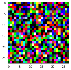
First of, we have to generate some random data to play with. As you may know, data is split into batches containing multiple data points. And because we have RGB data, we have three channels (Red, Green, Blue) and, in our case, a 28 x 28 pixel image. In sum, we have a batch dimension, a channel dimension, and two pixel dimensions:
torch.manual_seed(0)  # Fixing randomness for reproducibility

data = torch.randn(8, 3, 28, 28)  # 8 batch, 3 channels, 28x28 pixels
This is just random, nonsense data, but we can now inspect the first datapoint in our batch using Matplotlib:
import matplotlib.pyplot as plt

plt.imshow(data[0].permute(1, 2, 0))
Clipping input data to the valid range for imshow with RGB data ([0..1] for floats or [0..255] for integers).
<matplotlib.image.AxesImage at 0x7fee6fbc1280>
Optional: Why are we using permute to rearrange the data for matplotlib? What happens if you plot the data without permute?
Creating a model#
You may have seen models in PyTorch before. If so, this is quite straight-forward for you. If not, don’t worry. Think about the following code as a series of stepping stones laid out in front of you; to begin with, you simply jump onto the first stone, then to the next, and so on until you reach the final stone. These “stones” are layers in our network..
In this specific example we can imagine having a random picture we would like to classify (is it a bird? is it a plane?!). To do it, we simply just send it jumping through the layers. And for each jump, we narrow down the options. From animal to mammal to carnivore to bird etc. In broad terms, that’s how normal classification models work.
The only twist we have added is to use simulated, biological neurons. For technical reasons they are called Leaky Integrate-and-Fire (LIF) neurons. But in principle they are quite simple: they take some data, think about about it, and spit out a signal. Here’s how it works:
import torch.nn as nn
import norse.torch as norse

model = norse.SequentialState(
    nn.Conv2d(3, 6, 7, 1),
    norse.LIFCell(),
    nn.Conv2d(6, 12, 7, 1),
    norse.LIFCell(),
    nn.Flatten(1),
    nn.Linear(3072, 10, bias=False),
)
Now that we’ve defined our model, we can use it! Don’t worry if you don’t understand everything for now. You can always come back to study it in detail.
Optional: What happens if you try to print the model using print(model)? Can you explain the output?
3. Using the model#
output, state = model(data)
You are probably asking why there are two variables returned when model is being called. Good question! The output contains the actual data. But the state describes and keeps track of the current status of the neuron layer after we gave it the input data. Why? Because neurons change behaviour over time. Sometimes they’re active, sometimes they’re not. This is a topic for later tutorials - which you’re hopefully motivated to follow!
Now we can look at the output and the state respectively.
Inspecting the output#
For the output, we would expect 8 classification because we had 8 batches. That is, for every batch, we would expect one classification. How, then, does a classification look? If you, for instance, have 10 different types of birds you wanted to classify, you will need 10 outputs to indicate the likelihood for each type of bird. If the birds are, for instance [European Swallow, African Swallow, Segaull, Lark, Stork, ...] and you get the output [1, 0.2, -1.1, ...] then the network guesses it’s a European Swallow.
In our case, we are only using dumb, random data, so for now we only care about the shape of the output variable. That is, the size of what came out of our spiking neural network model. Because we have 8 batches and 10 classes, we expect a shape of [8, 10].
To validate our assumption, run this:
output.shape
torch.Size([8, 10])
Nice, it fits! We’ve successfully reduced the 8 images (3 channels, 28x28 pixels) down to 8 vectors of 10 numbers. This is, of course just a random example because our network is not trained yet. However, it’s already a big step: what’s great about these vector outputs (actually, they’re called tensors in many dimensions), is that they can be interpreted to mean almost anything. Birds, Handwritten digits, Voice commands, … You name it!
Inspecting the state#
We still have not looked at the state, you may (correctly) point out. The state keeps track of when the neurons fire. Without it, we wouldn’t know when to emit a spike (1) and when to stay silent (0).
I can already now tell you that the state of a neuron layer contains two things: the voltage v and the current i (after the SI symbols). We don’t have time to understand why they are called v and i, but it’s sufficient to know that they inform us about how close the neuron is to firing (emitting a 1). That is why we need the state.
“Wait”, you may think, “if the state keeps track of each neuron layer, we should have 6 states right”? Exactly! But, while it contains 6 elements, we actually only need states for the spiking neuron layers. The other non-spiking layers give the same output over time so they can be considered as having constant state or can be ignored to be stateless. Since we have two stateful layers (LIFCell layers) in our model, we only need to keep track of two states:
[x.__class__ for x in state]
[NoneType,
 torch._jit_internal.LIFFeedForwardState,
 NoneType,
 torch._jit_internal.LIFFeedForwardState,
 NoneType,
 NoneType]
Perfect! The final piece of the puzzle is to make sure that our model actually spikes.
Optional: What do you think the v and i looks like? Try to introspect their shape and explain why they have the shape they have. (Remember that state is a list containing two elements).
Training the model#
Our model is currently not trained and is like an irratic illbehaving kid: it won’t do anything you ask it to. Norse models are trained in the exact same way that PyTorch models are trained. So, if you are familiar with that, the above information about layer output and state management should be sufficient to get you going.
However, let’s give you an intuition about how the models are trained so you understand the principle.
To do that, we need to look closer at the output. Let’s isolate the first datapoint and ignore the other 7 batch entries for now:
Optional: Find out why we are using .detach. What happens if you remove it? Why?
plt.plot(output.detach()[0])
[<matplotlib.lines.Line2D at 0x7fee6fba4f10>]
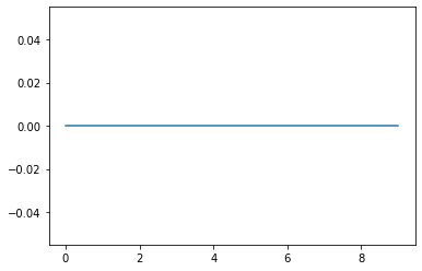
Gargh, that’s boring! It’s completely dead. Of all the 10 classes we predict, they’re all zero!
That’s because the neuron only received input during one timestep. That’s not nearly enough to make it spike. What happens if we try to give it multiple inputs, say, 32?
timesteps = 32
output = None
state = None
for timestep in range(timesteps):
    output, state = model(data, state)
plt.plot(output.detach()[0])
[<matplotlib.lines.Line2D at 0x7fee6fb14dc0>]
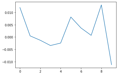
Much better! Now the network gave some output. The final linear layer makes it difficult to read exactly, but this, ladies and gentlemen, is a fully spiking neural network in the making. If this was a bird classifier model, it would definitely go for the European Swallow.
To train the network, we simply need to adjust our weights, like in normal PyTorch models. This is typically done via gradient based optimization which is outside the scope of this tutorial. Luckily, it’s easy to use and can be quickly explained: imagine that we are looking for a certain output of the model, say a spike. We can not take the difference between what we expect and what the model actually produced; that difference is how much the weights (\(w\)) in the model should change:
actual_output = output.sum()
expected_output = 1
difference = expected_output - actual_output
The only remaining thing is to use PyTorch’s clever optimization mechanisms to update the model so it learns to do better than before:
torch.optim.RMSprop
torch.optim.rmsprop.RMSprop
optimizer = torch.optim.RMSprop(model.parameters())  # Constructs the optimizer
difference.backward()  # Records impact of weights - see note on optimization above
optimizer.step()  # Takes a 'step' in the right direction
Reviewing the trained model#
Now that we “trained” the model, how does it look? Let’s try to run the model one more time and plot the outputs — just like before.
timesteps = 32
output = None
state = None
for timestep in range(timesteps):
    output, state = model(data, state)


plt.plot(output.detach()[0])
[<matplotlib.lines.Line2D at 0x7fee6faf9940>]
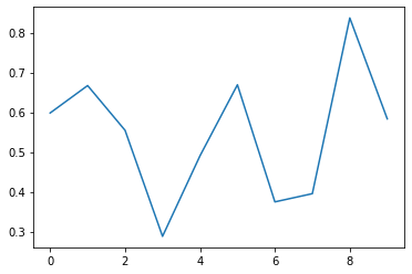
Granted, the model is not perfect. But look at the change in the y-axis. Something definitely happened!
Properly training a network takes many, many iterations with a good and representative dataset. That’s a topic for a different session and the summary section will point you to other notebooks that shows how to learn more challenging and exciting problems, like event-based vision, or reinforcement learning.
Optional: We did quite a bit of work to initialize variables, loop, and apply our model. This is actually already built into our LIF module. Try to rewrite the code above to use the LIF module instead of the LIFCell module. You can either re-work the entire model or just apply the data on a single LIF layer.
4. Summary#
You’ve succesfully built and trained your first Spiking Neural Network SNN (which you can use to classify birds!). As you’ve seen so far, training a SNN is just adding these special type of layers called spiking layers in a regular PyTorch Neural Network framework that have states which change over time. We train the network using regular gradiant based optimisation and BAM, it’s that simple.
We have plenty more resources in our notebook repository if you’re feeling adventurous. Also, our documentation tells you much more about what Norse is and why we built it at: https://norse.github.io/norse/
Don’t forget to join our Discord server and to support us by either donating or contributing your work upstream. Norse is open-source and built with love for the community. We couldn’t do it without your help!