Simulating and plotting neurons

Norse is a library where you can simulate neural networks that are driven by atomic and sparse events over time, rather than large and dense tensors without time.

Outcomes: This notebook is a quick introduction on how to simulate and analyse neuron activity,i.e, neuron activity over time. Specifically you will learn how to simulate single neurons and plot their voltage traces, current traces, and spikes.

Note

You can execute the notebooks on this website by hitting above and pressing Live Code.

Before you continue with this notebook, we strongly recommend you familiarize yourself with PyTorch (at least superficially). One way to do that is to go to their PyTorch Quickstart Tutorial.

---

Installation

First of all we need to install and import some prerequisites:

!pip install -q matplotlib numpy scipy tqdm git+https://github.com/norse/norse

^C
ERROR: Operation cancelled by user

import torch  # PyTorch

# Import a the leaky integrate-and-fire feedforward model
from norse.torch.module.lif import LIF, LIFParameters

Creating leaky integrate-and-fire (LIF) neurons

To start simulating we need to create a population of LIF neurons of an arbitrary size. Each neuron in the population is set to a default state. We will not be covering this particular neuron model in this tutorial; this tutorial is about learning how to visualise outputs from neuron layers. But you can find more information here and in our other tutorials.

Really, the only thing you need to remember is that that the neurons will receive currents as inputs, and produce spikes (0 and 1) as outputs.

# Creates a LIF population of arbitrary size
# Note that we record all the states for future use (not recommended unless necessary)
lif = LIF(record_states=True)
lif

LIF(p=LIFParameters(tau_syn_inv=tensor(200.), tau_mem_inv=tensor(100.), v_leak=tensor(0.), v_th=tensor(1.), v_reset=tensor(0.), method='super', alpha=tensor(100.)), dt=0.001)

1. Simulating a single neuron

To actually use the neuron, we need to simulate it in time. Why in time? Well, neurons works by integrating current over time. In Norse, time is discretized into steps, where each step advances the neuron simulation a bit into the future. If this confuses you, take a look at the earlier Tutorial on spiking neurons in PyTorch.

We can easily simulate a single neuron in, say, 1000 timesteps, that is 1 second by creating a tensor with 1000 zeros. Note that the time is the outer (first) dimension and the number of neurons is the second (last). In order for something interesting to happen we also inject input spikes at 100 ms and 120 ms.

data = torch.zeros(1000, 1)
data[100] = 1.0  # inject input spike at 100 ms
data[120] = 1.0  # and at 120 ms
output, states = lif(data)

The output now stores the output spikes and the states contain the internal variables of the neuron dynamics, such as the voltage trace.

Note

What does states consist of? What happens if you print it out?

And what happens if you go back to the previous cell and sets record_states=False?

Now, how can we tell what happens? We have chosen to record the output state, so immediately plot the voltage state with Matplotlib:

import matplotlib.pyplot as plt

fig, ax = plt.subplots()
ax.plot(states.v.detach())
ax.hlines(y=1.0, xmin=0.0, xmax=1000, linestyle="--", color="k")
ax.set_xlabel("Time [ms]")
ax.set_ylabel("Voltage")

Text(0, 0.5, 'Voltage')

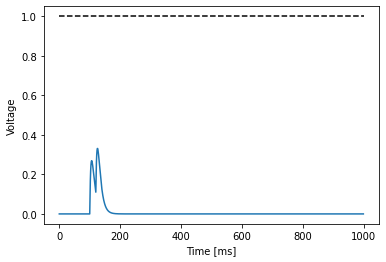
As you can see the neuron receives an input around timestep 100, which causes the neuron voltage membrane to react. However, the voltage trace does not reach the default threshold value of 1.0. Indeed we can compute the maximal value and timestep at which it is attained:

voltages = states.v.detach()
max_voltage = torch.max(voltages)
f"maximal voltage: {max_voltage} at {torch.argmax(voltages)} ms"

'maximal voltage: 0.33088549971580505 at 126 ms'

Note how that value is much below 1.0. Therefore we can simply rescale the input to ellicit at least one output spike (we also now only show the membrane evolution between 0 and 200 ms).

scaled_data = 1.001 * (
    data / max_voltage
)  # rescale data according to max voltage + some headroom just computed
output, states = lif(scaled_data[:200])

fig, ax = plt.subplots()
ax.plot(states.v.detach())
ax.hlines(y=1.0, xmin=0.0, xmax=200, linestyle="--", color="k")
ax.set_xlabel("Time [ms]")
ax.set_ylabel("Voltage")

Text(0, 0.5, 'Voltage')

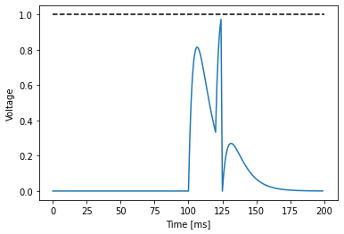
What happens here is that the neuron receives an input around timestep 100 - and again at 120. The neuron racts more strongly than before (the voltage values are higher). Around timestep 123, after the second current injection, the neuron gets sufficient momentum to elicit a spike. After the spike, the neuron resets, but there is some residual current that still produces an effect in the voltage membrane. Exactly why this happens is explained much better in the book Neural Dynamics by W. Gerstner et al.

As a small exercise, can you figure out how to visualize the current term ("i")?

2. Simulating multiple neurons

A nice feature of the fact that we are using pytorch is that we can easily simulate many neurons at the same time. Here we consider 10000 neurons over 1000 timesteps (that is one second). We do so by generating random spike input as follows

timesteps = 1000  # simulate for 1 second (1 ms timestep)
num_neurons = 1000

# expect ~ 10 input spikes per neuron
input_spikes = torch.rand((timesteps, num_neurons)) < 0.01

We can verify our expectation that there are around \(10\) input spikes per neuron by computing the sum of the spikes over time

input_spikes.sum(dim=0).float().mean()

tensor(9.8110)

… And by plotting the activity histogram

fig, ax = plt.subplots()
ax.hist(input_spikes.sum(0).numpy())
ax.set_xlim(0, 30)
ax.set_xlabel("Number of spikes")
ax.set_ylabel("Occurrences")

Text(0, 0.5, 'Occurrences')

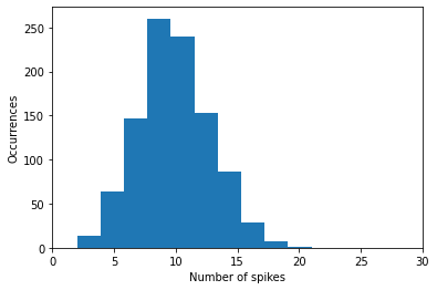
The histogram tells us that for our random data over 1000 timesteps, most neuron will receive 10 input spikes, less around 5 or 15 times, almost none will receive 0 or 20, and so on.

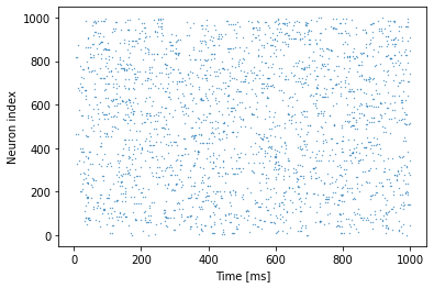
To run an actual simulation, we simply inject these input_spikes into our LIF neuron. This will provide an output of 1000 timesteps with 1000 neurons per timestep (so, a 1000x1000 matrix) and a state-variable, where the neuron states will be updated in. During the simulation, the states will update independently, resulting in different behaviours for every neuron.

lif = LIF(p=LIFParameters(v_th=0.3), record_states=True)
spikes, states = lif(input_spikes)

spikes.shape

torch.Size([1000, 1000])

We can visualise the spikes that the neurons produced as follows:

fig, ax = plt.subplots()
ax.scatter(*spikes.to_sparse().indices(), s=0.1)
ax.set_xlabel("Time [ms]")
ax.set_ylabel("Neuron index")

Text(0, 0.5, 'Neuron index')

We can compute the number of spikes per neuron again as follows

torch.mean(torch.sum(spikes, dim=0))

tensor(2.4740, grad_fn=<MeanBackward0>)

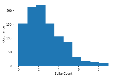
We gave different inputs to different neurons. For some neurons, enough to cause any spikes! For the other neurons, however, there are gradually more spikes as the input current increases.

We can inspect this spike pattern by summing up all the events in the time dimension and look at the activity histogram for the population:

fig, ax = plt.subplots()
ax.hist(spikes.sum(0).detach().numpy())
ax.set_xlabel("Spike Count")
ax.set_ylabel("Occurrence")

Text(0, 0.5, 'Occurrence')

3. Conclusion

Hopefully, this tutorial helped you gain some tools to plot spikes and neuron state variables and gave you some pointers on how to gain insights into spiking data in Norse. There are more primivites to explore for plotting that we did not get to, but they are relatively simple; the most important thing is to understand the shape and nature of your data, such that you can manipulate it in any way you need.

Additional resources

For an excellent introduction to neuron dynamics and much more, see the Neuromatch Academy Python tutorial.

---

We have plenty more resources in our notebook repository if you’re feeling adventurous. Also, our documentation tells you much more about what Norse is and why we built it at: https://norse.github.io/norse/

Don’t forget to join our Discord server and to support us by either donating or contributing your work upstream. Norse is open-source and built with love for the community. We couldn’t do it without your help!